Draw contour function of ternary simplex space

This example illustrates how to draw contourplots for functions with 3 probability inputs and multiple outputs.

# Author: Miquel Perello Nieto <miquel.perellonieto@bristol.ac.uk>
# License: new BSD

import matplotlib.pyplot as plt
import numpy as np
np.random.seed(42)

print(__doc__)

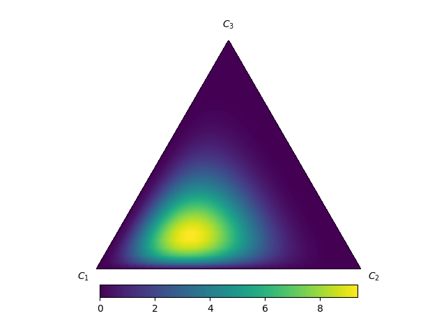
We show first how to draw a heatmap on a ternary probability simplex, in this case we will define a Dirichlet function and pass it with default parameters.

from scipy.stats import dirichlet

from pycalib.visualisations.ternary import draw_func_contours

function = lambda x: dirichlet.pdf(x, alpha=[5, 3, 2])
fig = draw_func_contours(function)

Next we show how do use a ternary calibration model that has 3 probability inputs and 3 ouputs. We will first simulate a calibrator by simulating 3 Dirichlet distributions and applying Bayes rule with equal prior.

class calibrator():
    def predict_proba(self, x):
        pred1 = dirichlet.pdf(x, alpha=[3, 1, 1])
        pred2 = dirichlet.pdf(x, alpha=[6, 7, 5])
        pred3 = dirichlet.pdf(x, alpha=[3, 4, 5])
        pred = np.vstack([pred1, pred2, pred3]).T
        pred = pred / pred.sum(axis=1)[:, None]
        return pred

cal = calibrator()

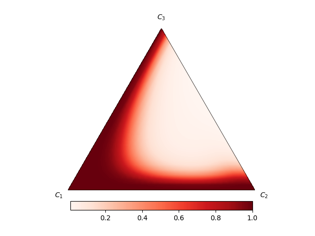
Then we will first draw a contourmap only for the first class. We do that by creating a lambda function and selecting the first column. We also select a colormap for the first class.

function = lambda x: cal.predict_proba(x.reshape(-1, 1))[0][0]
fig = draw_func_contours(function, cmap='Reds')

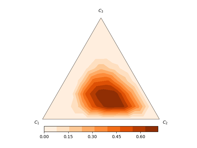
We can look at the second class by creating a new lambda function and selecting the second column. We will also modify how many times to subdivide the simplex (subdiv=3). And the number of contour values (nlevels=10).

function = lambda x: cal.predict_proba(x.reshape(-1, 1))[0][1]
fig = draw_func_contours(function, nlevels=10, subdiv=3, cmap='Oranges')

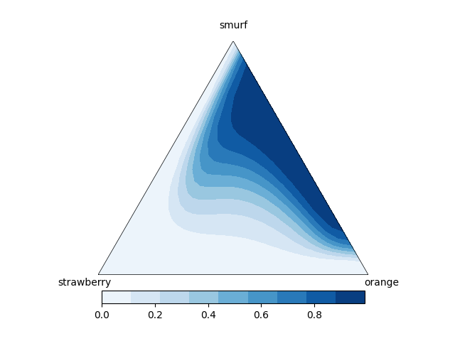
Finally we show the 3rd class with other sets of parameters and specifying the names of each class.

function = lambda x: cal.predict_proba(x.reshape(-1, 1))[0][2]
fig = draw_func_contours(function, nlevels=10, subdiv=5, cmap='Blues',
                         labels=['strawberry', 'orange', 'smurf'])

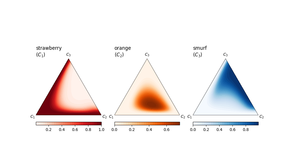
In order to plot the contours of all classes in the same figure it is necessary to loop over all subplots. We show an example that uses the previous functions.

labels=['strawberry', 'orange', 'smurf']
cmap_list = ['Reds', 'Oranges', 'Blues']
fig = plt.figure(figsize=(10, 5))
for c in [0, 1, 2]:
    ax = fig.add_subplot(1, 3, c+1)
    ax.set_title('{}\n$(C_{})$'.format(labels[c], c+1), loc='left')
    function = lambda x: cal.predict_proba(x.reshape(-1, 1))[0][c]
    fig = draw_func_contours(function, nlevels=30, subdiv=5, cmap=cmap_list[c],
                             ax=ax, fig=fig)